
|
PENCE / CIHR-Group
|

|
Funding for this software has been provided in part by the
Canadian Institutes of Health Research (CIHR Group)
and the
Protein Engineering Networks of
Centres of Excellence (PENCE).
|
|
PENCE / CIHR-Group
|
|
Funding for this software has been provided in part by the
Canadian Institutes of Health Research (CIHR Group)
and the
Protein Engineering Networks of
Centres of Excellence (PENCE).
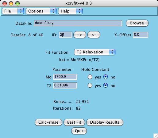
Purpose: A graphical X-windows program for binding curve studies and NMR spectroscopic analysis. Starting with version 4.x support for some functionality is provided for multiple datasets.
|
|
The power of xcrvfit lies in its convenience to process multiple datasets of various formats, the ability to experiment with fitting parameter scenarios, and the ability to customize the graphics. The program runs quickly and on any platform supporting X-windows. Output from the program includes a graph of the function through the data, the rmse of the fit, a measure of the sensitivity of each fitting function parameter, and a table showing how each datapoint fits the function. The current version allows users to overlay or place multiple fits on one plot.
xcrvfit: a graphical X-windows program for binding curve studies and NMR
spectroscopic analysis, developed by Boyko, R. and Sykes, B.D.  (University of Alberta).
website: http://www.bionmr.ualberta.ca/bds/software/xcrvfit
Copyright (C) 1994 - No portion of this program may be incorporated into other programs or sold for profit without express written consent of the authors.
Note:
It is assumed your operating system is supporting tcl/tk. Older systems
may not have this support but you can find/download it easily from the
internet. If you type "wish" in a terminal window and get "command not found"
then you will need to address this issue first before trying xcrvfit.
Note:
To save xcrvfit plots in png/tiff format you may also need to install the
tcl Img package. On my machine, I get this functionality by using an
enhanced version of tcl called activetcl which is available
on the internet.
You will need to download and install this package.
Either double click the xcrvfit icon (aqua version) or type xcrvfit
in a terminal window.
If you do not get a graphical window, make sure the software was
installed correctly.
Optional: You can also give command line arguments if you start xcrvfit from a terminal
window. Here is a brief description of the arguments.
Use the entry box provided or use the "Browse" button
to find it in your file system.
Here is example data that you can use.
More example data can be found in the Fitting functions
section.
For an explanation of the various
data formats that xcrvfit recognizes see the
Input Files
section.
If you do not see a plot, press the return or enter key in the Data File field.
The program displays the first data set by default. To display a
different dataset, most users prefer to click the Next or Previous buttons.
Click and hold the button currently labelled "Line" and select from our
current collection of functions.
For a more detailed explanation of these functions see
Fitting Functions .
Once the function has been selected, the program displays the
appropriate parameter fields. Some functions to the data being fitted, if this
is your first use of the program select the default "Line".
Calc-rmse stands for calculate root mean square error.
A graph of the fitting
function is displayed along with a root mean square error value.
If you do not see the fitting function, it could be that your starting
parameters are not very close. Set a=1 and b=1 if you are treating this section
as a tutorial.
Some functions will converge to the best fit function regardless of
the starting parameters. Others are very sensitive and a close
approximation is required first. If you have difficulties getting
convergence try holding one of more parameters as a constant.
Here you can see how every datapoint corresponds to the fitting
function. Also, you can see how sensitive each fitting parameter
is by looking at the StdDev field.
In this format the x-values are placed on the first line
and each subsequent line contains an identifier (likely the amino acid
number) and the corresponding y-values.
Any entry preceded with a "#" is treated as a missing value in
the table.
This format refers to Varian's vnmr 'fitspec.data' file format.
Here is an
example of this format.
This format refers to Varian's vnmr 'fp.out' file format.
An example of this format is found
here .
The log file "xcrvfit.log" contains a record of each convergence
achieved through pressing the iterate button. This is particularly
useful for stepping through a number of T2 fits.
Here is an example results file.
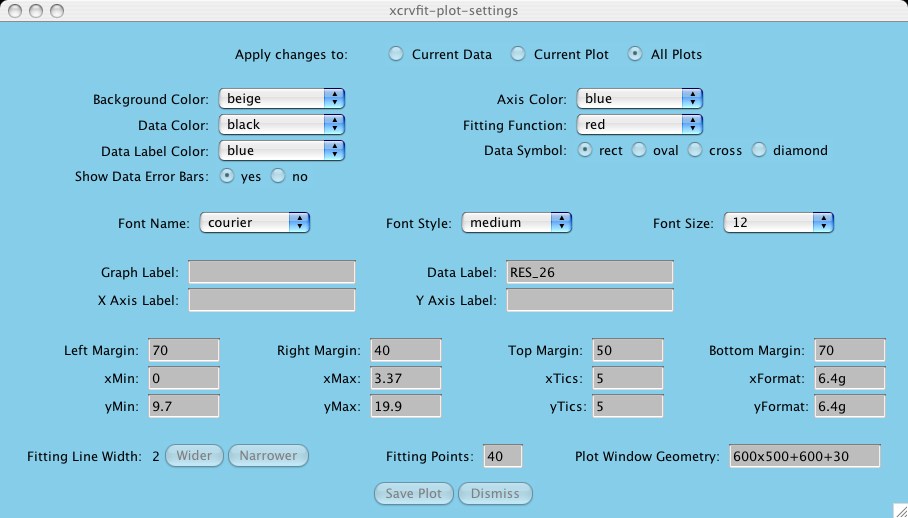
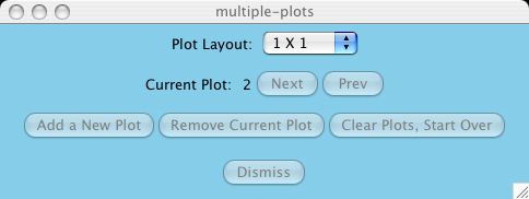
Under settings you can select the name of the plot you wish to customize.
The following window shows all the options you can change (the defaults are
read in from the lib/defaults/X11.defaults file).
Most of the items are self-descriptive. Here are the ones that may require
some explanation:
This means the user can relegate a change to a particular curve within a
plot or a particular plot within a set of plots. First the user needs to
define the current data or plot via the
Options -> Data Overlays -> Set Current Data or
Options -> Multiple plots -> Current Plot buttons in order to limit
the extent of the attribute change.
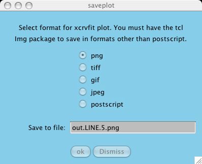
Saving a plot means you probably have to add some extensions to the
tcl/tk language. The default tcl/tk installation will support postscript
but this is not an effective solution for publication. Also, mac os x tends
to have problems with converting the generated tcl/tk postscript files to pdfs
(although using the ps2pdf utility seemed to work for me). So if you intend to
use the xcrvfit plots for publications, get the extensions!
There are several places to download and install Tkimg
like sourceFourge.net or activeTcl from ActiveState.
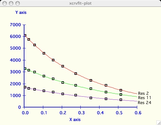
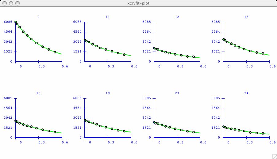
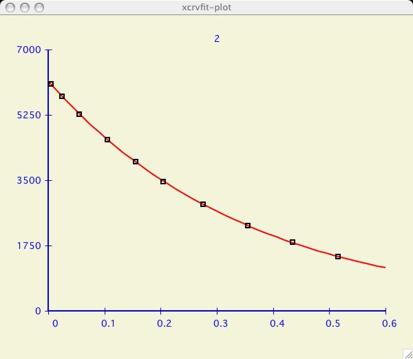
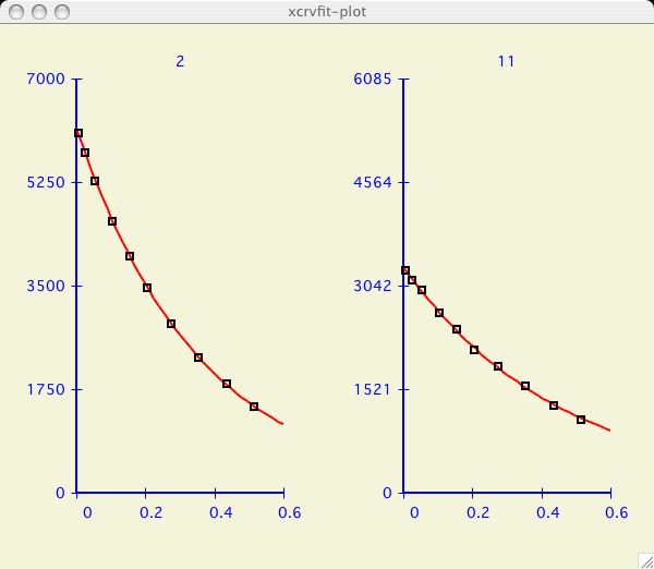
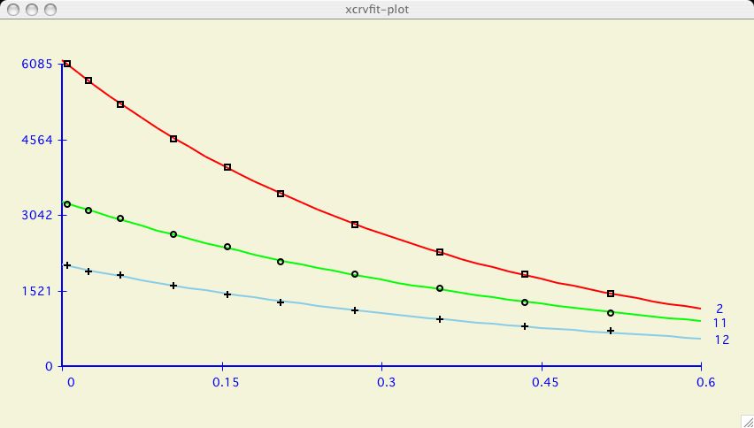
It can be very informative to visually compare the fits of several datasets.
I have chosen an example dataset with multiple data
( T2_RELAX )
and proceeded to fit the dataset labeled 2 as in the
first plot above. Now I am interested to compare the next dataset.
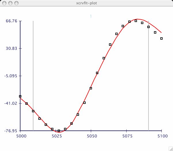
The only purpose of this option is to allow the user to cut the tails off a
a dataset before fitting. Sometimes the beginning or end of our data
acquisition, the user realizes that the data may be poor quality or noise.
Once the Options->Select Data Range window is invoked, the user clicks
the Increase/Decrease buttons until the appropriate data range is found.
If the user hits the Best Fit button, only those data between the range
bars are used in the calculation. In the example above, you can see how the
the outlier points can affect the final fitting function curve.
It can be very informative to visually compare the fits of several datasets
on one plotting axis. It is also common to display graphs in this format for
publication.
To demonstrate, we have chosen the
( T2_RELAX ),
example dataset which has multiple data in
( kay ) format.
What happens if I make a mistake and want to change some attribute
involving a previous dataset?
Use the Data Overlays->Set Current Data button to
select this dataset. You can tell which dataset is current because the data
flashes in the plot whenever the button is pressed.
Most researchers will have one dataset where the best fit of a particular
function indicates the best choice of a parameter of interest. But what happens
when the user has several valid datasets that essentially model the same
process? Reporting the key parameter of function becomes a complex
issue as it is unclear which data to consider and how important that dataset is
in relation to others in that family.
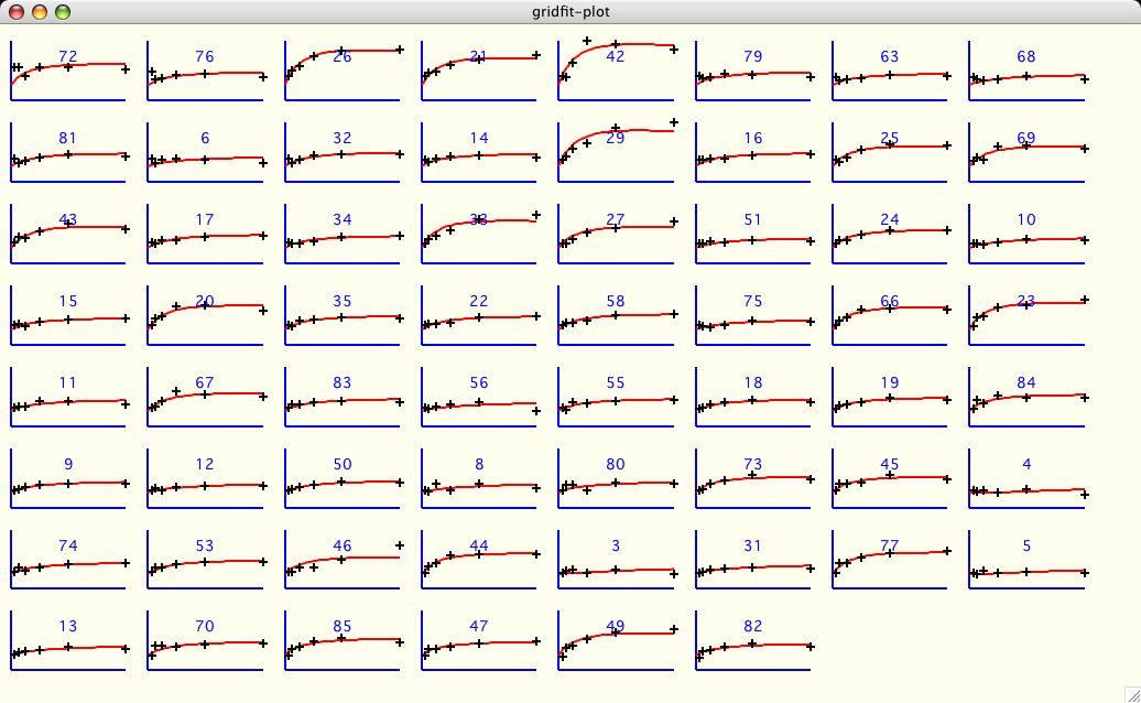
The intent of this section in xcrvfit is not to simplify the above process.
The software tries to present the results in a manner that allows the
researcher to make the best decision possible. Here is an example using the
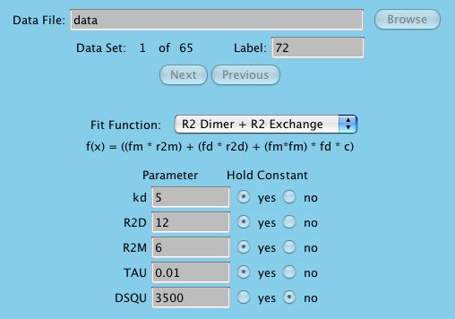
R2X_DIMER function using several amino acid datasets in search of
reporting the global value of kd. Although this is a specific example,
it should be clear how we can apply this technique to any function.
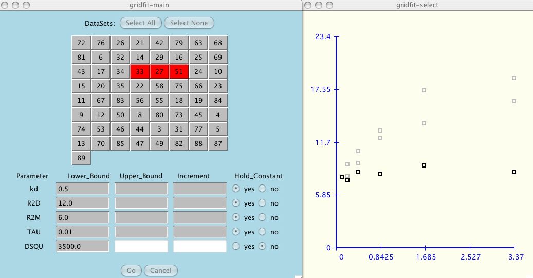
Next, as the user adds each dataset to the test suite, the data is shown in the
accompanying graph window (shown in black). The other data that you have
selected, if not current, is shown in grey.
This is a relatively effective and easy
way for the user to evaluate the credibility of each dataset
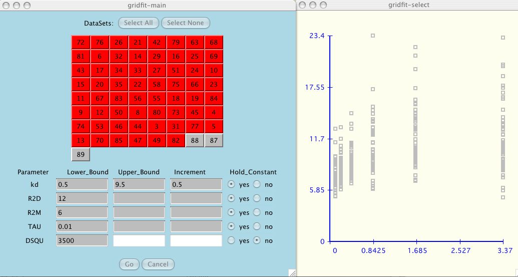
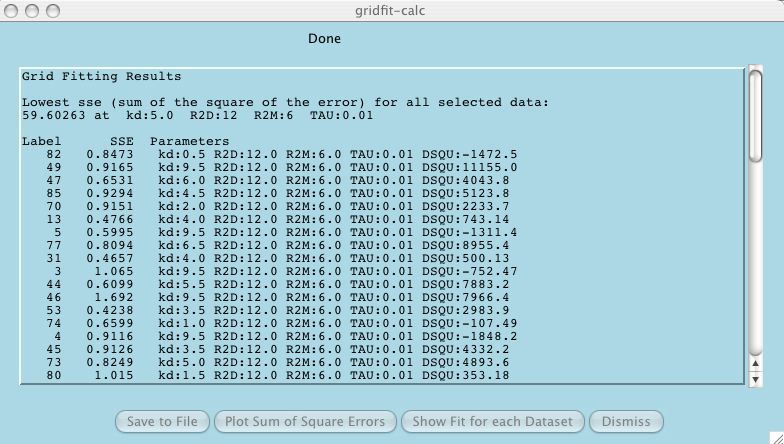
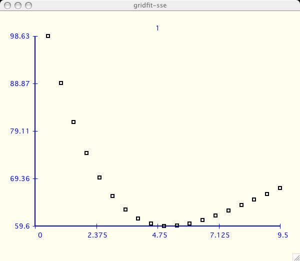
in the test suite. Some users will select Parameter Grid Fitting for
this function only!
At any time the user can include/exclude
all the datasets by clicking Select All or Select None.
If you have several datasets like this you probably want to
resize the window as big as possible. Also don't forget you have the
Settings->Plot Settings for gridfit-plot
menu option which allows you format and
save this output in the nicest way possible for publication.
The default settings in xcrvfit are set to maximize the space of each curve.
If you only have a few curves you may want to add scales and more space
between plots.
Problems and Issues
This file last updated:
Questions to:
bionmr@biochem.ualberta.ca
Download
Select the version of xcrvfit corresponding to your operating system.
We are no longer supporting sgi computers.
Installation
alias xcrvfit /home/rbo/xcrvfit-v4.0.12/bin/xcrvfit
Basic Usage and Tutorial for New Users
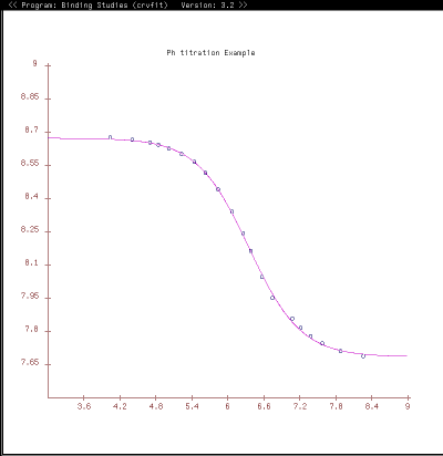
xcrvfit [datafile] [dataset] [function] [function parameters]
	 datafile  = your data file
	 dataset  = the label identifying the dataset in your data file
	 function  = the fitting function name to use (eg, PH_TITR)
	 function parameters  = starting values for the function.
	Fixed Parameters are preceeded with the keyword "const".

> cd my_data_dir
> xcrvfit test1.data A21 R2X_DIMER  5 const 12 const 6 const 0.01 3500
Input Files
The xcrvfit program can read data files which are in
one of the following formats.
Note: The kay, jfit and fp formats are automatically
converted to the crvfit format internally by the software.
	#
	# Example 2 column data in crvfit format
	#
	# x     f(x)
	#
	1.0    5.1
	2.2    12.0
	3.6    19.3
	5.0    30.4
Other examples of note include the
three column data for the XY2 function
where f(x) is dependent on x and x2.
	#
	# Example multiple dataset to fit function LINE
	# where each dataset is preceeded by a label character string
	#
	ALA_5
	1.00    -4.02
	2.00    -1.90
	3.00    0.23
	4.00    2.78
	5.00    4.34
	6.00    7.30
	MET_9
	2.00    4.50
	3.00    4.01
	4.00    4.79
	TYR_33
	1.00    2.50
	2.00    4.01
	3.00    8.79
Here is a simple example where only an error on f(x) is specified.
	#
	# Example input file with specified measurement errors
	#
	# x    y        xlb xub ylb yub
	#
	1.0    5.1      0.0 0.0 1.0 1.0
	2.2    12.0     0.0 0.0 2.0 2.0
	3.6    19.3     0.0 0.0 3.0 3.0
Currently the specification of measurement errors does
not affect any of the algorithms used in best fitting. It is simply a visual
aid that can help a user to evaluate the legitimacy of proposed fits. This
visual aid can be turned off/on via the settings menu.
	#
	# Example of kay style input format
	#
	11.1 22.2 44.4 88.8 177.6 355.2 710.4 1420.8
	A3   4680    4390    3980    3450    2940    2100    1010     369
	V4   8670    8250    7870    6730    5560    4030    1880     436
	E5  13800   13500   12500   11000    8790    5930    2800     641
Here is another example with
numeric labels and one with
with missing data values .
Understanding the Output
Data Input.: data.cubic
Num of data: 10

Function...: Cubic Polynomial
Description: Notes: A0*x*x*x + A1*x*x + A2*x + A3
Parameters.: 4

Parameter   Hold Constant          Value         StdDev
A0.......:       no             -0.00506        0.00211
A1.......:       no              1.30573        0.13435
A2.......:       no             -5.14197        2.32052
A3.......:       no              8.09954       10.43368

Stddev.....: 9.5043
Iterations.: 116
Max It.....: 200

Point by Point Analysis
          X[i]           Y[i]         Y-Calc       Residual
       0.00000        2.00000        8.09954        6.09954
       4.30000       13.00000        9.72971       -3.27029
       9.60000       93.00000       74.59546      -18.40454
      14.70000      190.00000      198.59236        8.59236
      18.70000      319.00000      335.45210       16.45210
      23.30000      537.00000      533.14359       -3.85641
      27.50000      750.00000      748.90418       -1.09582
      32.40000     1044.00000     1040.07185       -3.92815
      36.80000     1340.00000     1334.93300       -5.06700
      41.80000     1700.00000     1704.96881        4.96881
Customizing and Saving Your Plots
Multiple Plots
Select Data Range
Multiple data on One Plot
Parameter Grid Fitting
Appendix: Older Versions of xcrvfit
The following programs were all pre-cursors which led to the development of
this current version of xcrvfit.
Crvfit
Crvfit was developed at the University of Alberta in the Brian Sykes
lab in 1989 on a sun using sunview.
Crvfit was frequently used in the lab for binding curve studies where
some functions are of the form f(x, x2). We also used crvfit to
calculate T1 and T2 relaxation curves and J coupling constants.
Fast Crvfit
Fast crvfit is a derivative of crvfit which fits multiple input
files to the same function. So if you have lots of data files
that you wish to fit with the same function, this program could
save alot of time. However it is a risky program in that there
is no graphical output. You will not be able to "see" the fit,
the output is a statistical report only. Fast crvfit was written in C and
later became the back-end software for xcrvfit.
CrvfitS
This program does curve fitting for binding studies for
the following cases:
However this program was written with sunview graphics and there was not
enough impetus to port it to X-windows.
Crvfit_nmrdata
This is a small utility which reformats our vnmr data files
to crvfit or jfit data files.
Dimerfit
This program finds chi-square values from fitting data to curves
by varying the values for kd1, kd2 and kdimer. There is also
an option which allows the user to have the output formatted
into a table which is acceptable for input into the
macintosh "wingz" program.
Jfit
Graphical curve fitting package for estimating J-coupling constants
via absorption/dispersion Lorentzians or Gaussian functions.