 |
xcrvfit Brian Sykes Lab |
 |
| |
xcrvfit Brian Sykes Lab |
|
Version: 5.0.3 - Jun 2012
Download and Installation
Purpose: A graphical X-windows program for binding curve studies and NMR spectroscopic analysis.
|
|
The power of xcrvfit lies in its convenience to process multiple datasets of various formats, the ability to experiment with fitting parameter scenarios, and the ability to customize the graphics. The program runs quickly and on any platform supporting X-windows. Output from the program includes a graph of the function through the data, the rmse of the fit, a measure of the sensitivity of each fitting function parameter, and a table showing how each datapoint fits the function. The current version allows users to overlay or place multiple fits on one plot.
Authors:
Robert Boyko,
Brian Sykes
This software is inhouse and currently not published. You can reference it
in the following fashion for now:
xcrvfit: a graphical X-windows program for binding curve studies and NMR
spectroscopic analysis, developed by Boyko, R. and Sykes, B.D.  (University of Alberta).
website: http://www.bionmr.ualberta.ca/bds/software/xcrvfit
Copyright (C) 2012 -
No portion of this program may be incorporated into other
programs or sold for profit without express written consent
of the authors.
Linux - Same as the macosx procedure but you may have to
explicitly drag the directory from the opened window to the desktop.
If you do not get an xcrvfit folder, then un-tar the download file
(eg, tar xvf xcrvfit*.tar) and move it to your Desktop.
Double click the xcrvfit icon or
see these notes for command line usage.
If you do not get a graphical window, re-visit the installation section of this manual.
Use the entry box provided or use the "Browse" button
to find it on your file system.
Here is example data that you can use.
For an explanation of the various
data formats that xcrvfit recognizes see the
Input Files
section. Use the view button to verify your input data file.
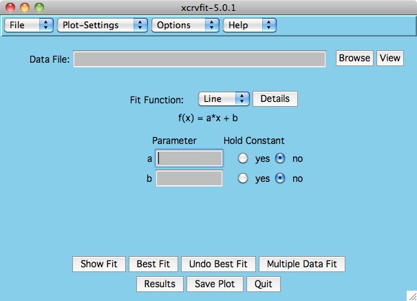
Click and hold the button currently labelled "Line" and select from our
current collection of functions.
For a more detailed explanation of these functions see
Fitting Functions .
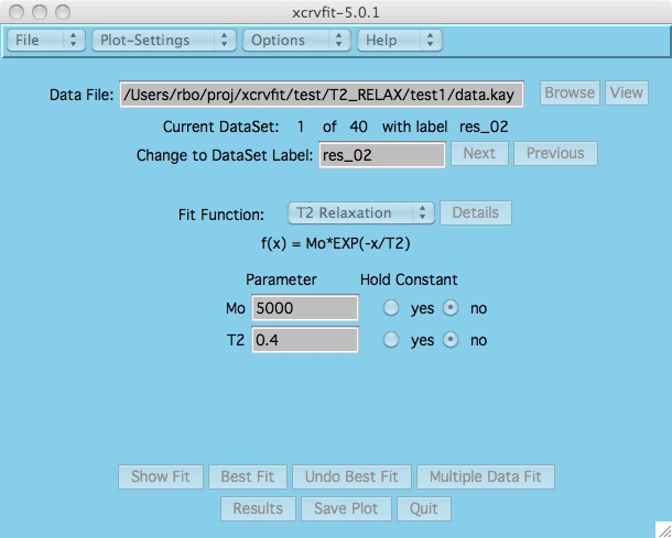
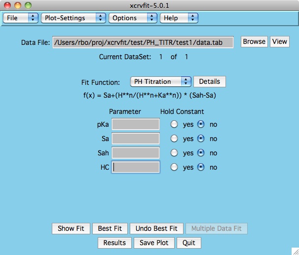
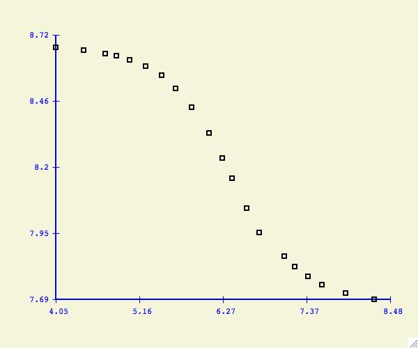
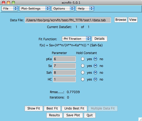
Once the function has been selected, the program displays the
appropriate parameter fields.
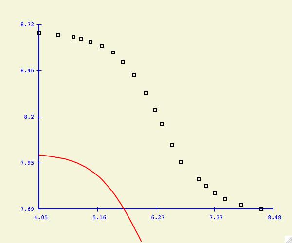
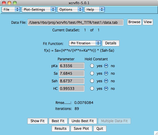
A graph of the fitting
function is displayed along with a root mean square error value.
If you do not see the fitting function, it could be that your starting
parameters are not very close.
Some functions will converge to the best fit function regardless of
the starting parameters. Others are very sensitive and a close
approximation is required first. If you have difficulties getting
convergence try holding one of more parameters as a constant.
Here you can see how every datapoint corresponds to the fitting
function. Also, you can see how sensitive each fitting parameter
is by looking at the StdDev field.
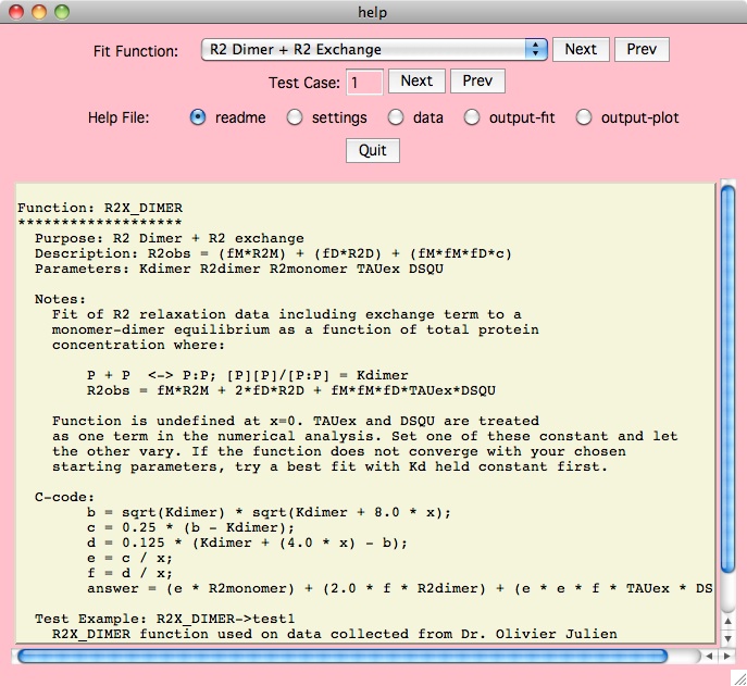
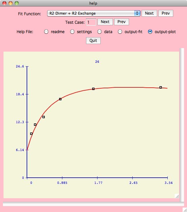
However you will likely find that the
Details button next to the Fit Function on the main panel
is the best way to figure out the xcrvfit functions. Here we may show you
multiple test cases for each specific function, where each test case
includes the readme files, input data, output files and plots,
and application defaults files (which allow you to understand how we got
the results we did).
All the examples presented here are those that are found in
our examples download .
Example 1 :
In the simplest case, the text file contains only one dataset. The x-values
are in column 1 and y-values in column 2 with at least one white space
character separating each number.
Example 2 :
Some functions require the input of second independent variable. For
eample, the XY2
function which models titration data takes into account the measurements
of protein dilution.
Any secondary x-values are entered in the 3rd column.
Example 3 :
Multiple datasets can be placed in one file however an identifying label
must be found on the line preceding each data set. The alphanumeric
label cannot have spaces (white space).
Example 4 :
It is also possible to specify measurement errors for any or all data points.
Following on the same line as the data point, the following four
data columns are specified:
Example 5 :
Older versions of xcrvfit sometimes had issues reading data files
created on MS Windows because of control M characters at the end of each
line. This issue should now be resolved.
In this format the x-values are placed on the first line
and each subsequent line contains an identifier (likely the amino acid
number) and the corresponding y-values.
Any entry preceded with a "#" is treated as a missing value in
the table.
Example 6 : note that
identifier (first column) can be either numeric or a label
Example 7 :
with missing data values
This format refers to Varian's vnmr 'fitspec.data' file format.
The first entry is the number of points, the second is start of
plot, the third is width of plot. The following lines contain
each y-value, one per line.
Example 9 :
This format refers to Varian's vnmr 'fp.out' file format.
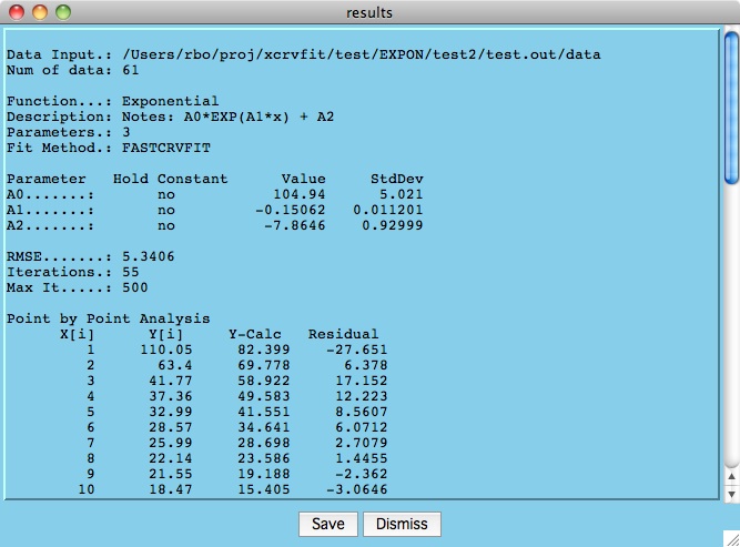
Below is an example results file that is generated when the user
hits the Best Fit button and convergence is achieved. Here
we can see the total root mean square error of the data to the fitting
function as well as the values/error estimates for the parameters.
The "Point by Point Analysis" indicates the difference between the
calculated and measured y-values.
Click the Save button
to write the results to a file you specify.
Click on File->Save Current Settings and the software asks you
where to save these defaults. The most logical place to save your settings is
in the same directory as your data input. Do this and
call it xcrvfit.defaults.
If you want to start xcrvfit by clicking on an icon, say in
/Applications, then how will the software know where to read in your saved
defaults? In this case, take a close look at the
examples data that comes with the software . Copy
xcrvfit.command to the directory that contains your data and run this
command (either in a terminal or clicking on the icon).
This is the best way to organize your multiple xcrvfit runs.
However,
if you insist on taking a more short-sighted view, you can save xcrvfit
preferences to $HOME/.xcrvfit.defaults. Now when you click the
xcrvfit icon and it will read your preferences.
Here are some of the most common edits people may wish to make
on the xcrvfit.defaults file:
Most of the items are self-descriptive. Here are the ones that may require
some explanation:
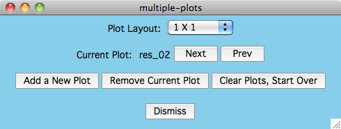
The Next and Prev buttons are used to select the current plot.
You can tell which plot is current because the data
flashes in the plot whenever the button is pressed.
Once you have selected a current plot, you can Remove Current Plot
or you can click the Plot-settings -> xcrvfit-plot menu item
to make plotting parameter changes which apply only for this plot.
For small numbers of plots, you can use the Plot Layout menu item
to manually set the dimension for the plots in the plotting window. The
default Plot Layout is to increase the number of columns by one
whenever the row and column values are equal. If we need another plot and
we have more columns than rows, then we draw the next plot in a new row.
What happens if I make a mistake and want to change some attribute
involving a previous dataset?
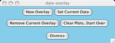
Use the Data Overlays->Set Current Data button to
select this dataset. You can tell which dataset is current because the data
flashes in the plot whenever the button is pressed.
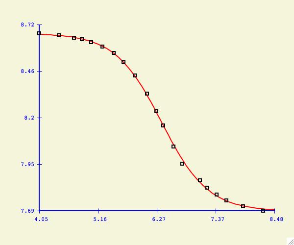
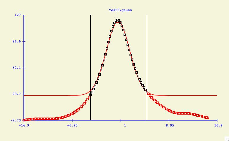
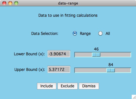
The purpose of the Options -> Data: Select Range menu item
is to allow the user to change what y-values are included/excluded from
the curve fitting process. As shown in the plot above, this could mean
cutting the tails of noisy data, or it could also mean the elimination of
data points which are suspect of being in error.
To understand how to mimic the plot above, start by bringing up the
data-range window.
First we eliminate all the data points by
clicking the All radio button and followed by the Exclude button.
Then we click the Range button and use the mouse to move both slider
buttons to determine the area of the curve that we want to fit. Press the
Include button and now all points used in the fitting calculation are
displayed in black. Finally click the Best Fit button to see how
this graph looks when compared to fitting all the data.
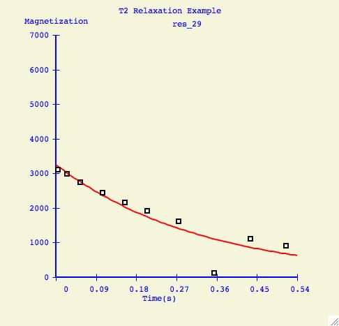
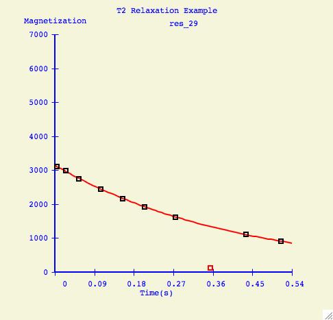
To elimate specific points from the fitting calculation, the user selects
Range, positions the sliders, but this time presses Exclude.
Here is an example of a how a fitting curve may look before and after we
have excluded the possibly erronous data point.
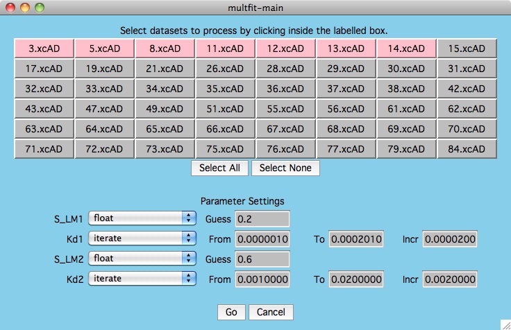
First, read in your multi-dataset datafile and set the fitting
function. Click on the Multiple Data Best Fit button and you are
presented with the first window below.
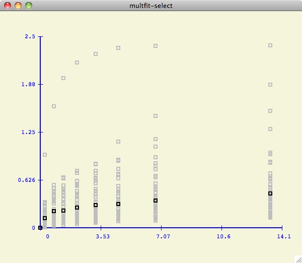
For this particular test, we are interested
in the values of kd1 and kd2 that best fit all the data we selected.
As shown below, we have decided to only consider the first 7 datasets
(hilited in pink). Note that the multfit-select window is drawn to
help the user visualize how the current dataset values compare to the others.
Since the data is in kay format, the x-values are all the
same for each y-value (that is why all the data values are stacked in distinct
vertical lines).
This is a relatively effective and easy
way for the user to evaluate the credibility of each dataset
in the test suite.
Then we give initial values to S_LM1 and S_LM2 and by specifying "float"
we allow the fitting algorithm to choose these parameters to minimize the error
in the fitting function for each particular dataset. Meanwhile, we are
interested in not only holding kd1 constant, but that constant will start at a
lower bound and will be stepped up by an increment until the upper bound
is reached. The same is done for kd2. Press the Go button to enable
the calculations.
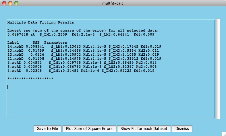
The window presented below is the output from the calculations where we
can see the best fitting parameters for the chosen datasets.
The top set of numbers indicates the overall lowest sum of squares of error
for all our selected residues. This is achieved somewhere in the
vicinity of kd1=2.1e-5 and kd2=0.009 (remember we taking relatively large
steps between values of kd1 and kd2).
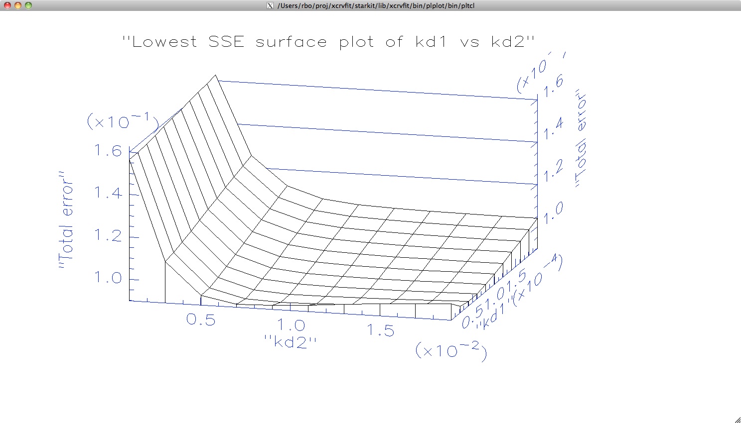
At this point it is interesting to see a plot of total error at each kd1,kd2
pair. In order to do this, the xcrvfit software has been written to use
the scientific plotting package
plplot .
The plot
is shown when the user clicks Plot Sum of Square Errors.
Here we can get a sense of the trough in the surface plot where values
of kd1 and kd2 give essentially the same solution to the fitting problem.
The plplot
software is capable of producing many types of 3D plots, however we have
only written a module to encorporate surface plots.
Also plplot
may be complex to install
for some users so we have included an executable version (5.9.9)
within the xcrvfit application.
The xcrvfit
software presents a limited number of settings for configuring the
3D plot under Plot-settings -> multfit-3d. Contour plots are
currently not supported and to change the point of view for viewing
the surface plot, try changing values for Surface Plot Alt
and Surface Plot Azimuth.
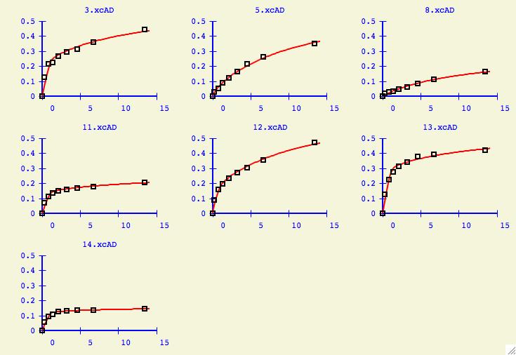
Finally users will be interested to see what kinds of plots are
generated for the individual datasets using the overall
best values of kd1 and kd2. Press the Show Fit for each Dataset
button to get the window below. In this particular case, all the datasets
can be fit quite nicely without any outliers.
Note that you will probably want to change
some of the Plot-Settings -> multfit-plot options and save the
changes with File -> Save Current Settings .
At this point, click on the Show Fit for each Dataset button and now
we can effectively analyze how our global best fit at kd1=.0001, kd2=.009 works
with each individual dataset. Do some datasets not fit well and why might that
be?
This file last updated:
Questions to:
bionmrwebmaster@biochem.ualberta.ca
Download and Installation
Basic Usage and Examples for New Users
Fitting Functions
Here is
a summary description of all the fitting functions in this version of xcrvfit
.
Input Files
The xcrvfit program can read data files which are in
one of the following formats.
Note: The kay, jfit and fp formats are automatically
converted to the crvfit format internally by the software.
Currently the specification of measurement errors does
not affect any of the algorithms used in best fitting. It is simply a visual
aid that can help a user to evaluate the legitimacy of proposed fits. This
visual aid can be turned off/on via the settings menu.
Output Files
First, xcrvfit tries to figure out the name of the directory
which contains all the output files. If the user provides no information
about this, then the default place is $HOME/Desktop/xcrvfit_out .
It is usually good practice to specify the output directory in the
xcrvfit.defaults file.
Settings and Preferences
It takes a fair amount of work to setup xcrvfit. You have to tell the
software where the data is, the fitting function and reasonable starting
values, or even change plotting variables to get the nicest looking plot
possible. Once you have it, you do not want to do it again.
# where is your data file  (can be full pathname)
*data_file:     data.fp

# where is your output directory (can be full pathname)
*output_dir:    xcrvfit_out

# Selected function and starting parameter values
*func_key:      EXPON
*func_parms:    100.0:-0.1:-8

# customize graphing parameters to get a nicer looking fit/data plot (plot 0)
*y_min_0:       -20.0
*y_max_0:       120
*y_tics_0:      8
*x_min_0:       0.0
*x_max_0:       70.0
*x_tics_0:      8
Customizing Your Plots
Under the menu item Plot-Settings you can select the name of the plot you wish to customize.
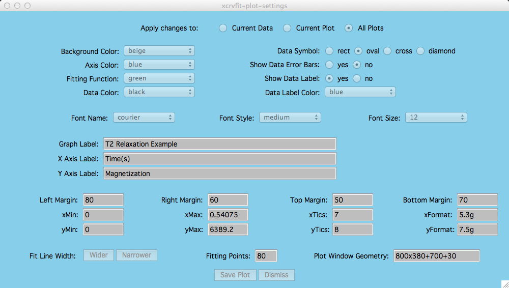
This option applies if you have several plots in one plotting window and
you only want to control attributes for a specific plot.
First the user needs to
define the current data or plot via:
Options -> Data Overlays -> Set Current Data or
Then by clicking Current Plot the extent of any attribute changes
within the Plot-Settings window applies only to that plot.
Options -> Multiple plots -> Current Plot
If measurement errors have been
included in the input file, then these are drawn along with the data points.
This is the title of the current dataset
and it is typically dragged by the user near the fitting curve for that dataset.
If you drag a title and re-size the graph, the location of the title will
revert back to its default setting.
Changing these attributes allows the user to nicely fit a single
plot in a window or get the right spacing between plots in a multiple
plot window.
These allow the user to specify how the axis
numbers are labelled (printf format).
For example, "5.2f" means print a
floating point number with width 5 characters and 2 numbers follow after the
decimal point. Type man printf for all the details, there are a lot of
possible formats.
The number of fitting points can be increased if more points
are needed to define the fiting curve. However it takes more time to compute
more points. Also this will not solve aliasing problems with curve display. In
fact, curves may look more natural with fewer points chosen (80 seems to
be about right).
This allows the user to manually set the
graphics window size and location. Most users, unless they need a specify
size of plot, will use the mouse to resize the plot window to the proper
viewing size.
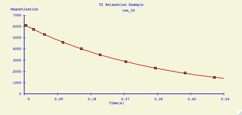
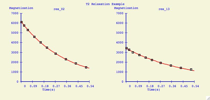
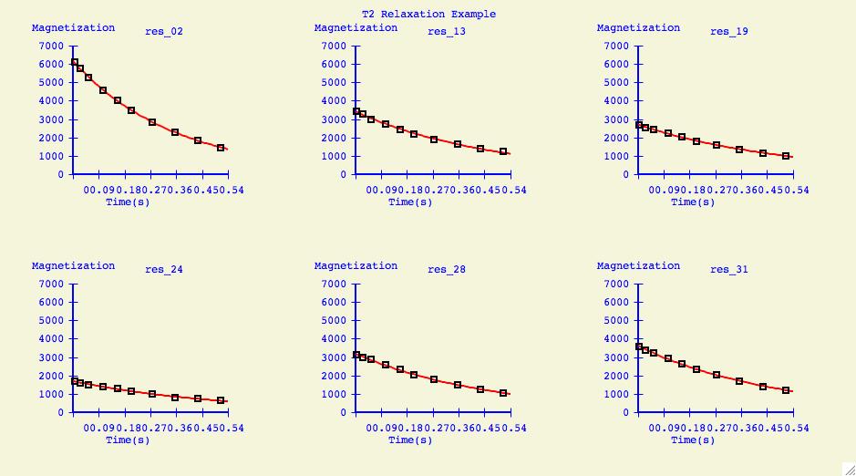
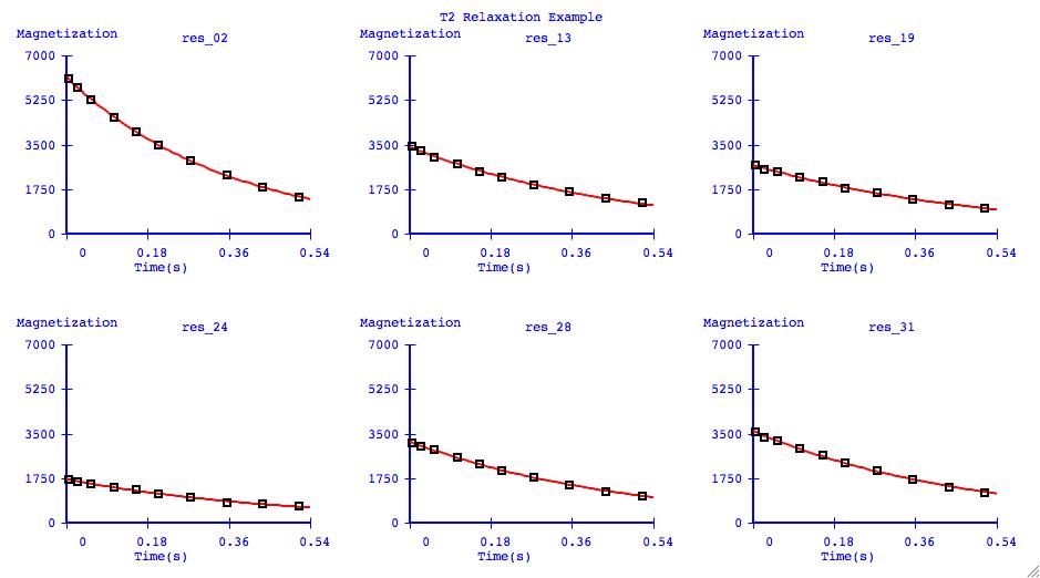
Multiple Plots
The purpose of this option is to individually arrange a number of
dataset fits into one plotting window for easier comparison.
Below is an example of what can be created for publication or
presentation purposes.
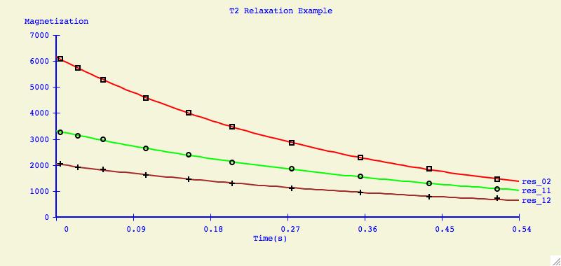
Data Overlays
It can be very informative to visually compare the fits of several datasets
on one plotting axis. It is also common to display graphs in this format for
publication.
Data Exclusion
Parameter Grid Fitting
What happens
when the user has several valid datasets that essentially model the same
process? The xcrvfit software has a special way to model one or two
parameters which are held
constant at various levels on all the data,
and then report the value of the parameter(s)
which had the least total error over all the datasets.
Appendix: History of xcrvfit
Crvfit
Crvfit was developed at the University of Alberta in the Brian Sykes
lab in 1989 on a sun using sunview.
Crvfit was frequently used in the lab for binding curve studies where
some functions are of the form f(x, x2). We also used crvfit to
calculate T1 and T2 relaxation curves and J coupling constants.
Fast Crvfit
Fast crvfit is a derivative of crvfit which fits multiple input
files to the same function. So if you have lots of data files
that you wish to fit with the same function, this program could
save alot of time. However it is a risky program in that there
is no graphical output. You will not be able to "see" the fit,
the output is a statistical report only. Fast crvfit was written in C and
later became the back-end software for xcrvfit.
CrvfitS
This program does curve fitting for binding studies for
the following cases:
However this program was written with sunview graphics and there was not
enough impetus to port it to modern computers.
Crvfit_nmrdata
This is a small utility which reformats our vnmr data files
to crvfit or jfit data files.
Dimerfit
This program finds chi-square values from fitting data to curves
by varying the values for kd1, kd2 and kdimer. There is also
an option which allows the user to have the output formatted
into a table which is acceptable for input into the
macintosh "wingz" program. This program was the forerunner to the
Best Fit Multiple Data option in xcrvfit.
Jfit
Graphical curve fitting package for estimating J-coupling constants
via absorption/dispersion Lorentzians or Gaussian functions.