1. Go to the stc installation directory and in lib/examples you will see a directory called basic . Copy this directory to your home directory.

2. List the directory and you will see there are two structures, jrb.complex.pdb and jrb.free.pdb Start the stc program by typing "stc".

   > cd tutorial 
   > ls
   > stc
   

   

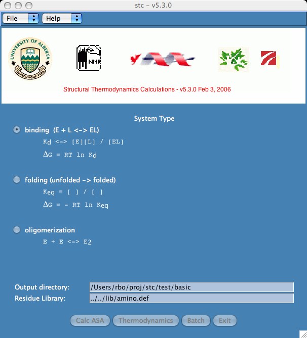
   Note that the system type for our data is "binding". One could also choose "unfolding" or "oligomerization". Our examples library contains sample runs of these system types.

   The output directory is where stc writes all the output files. The residue library is where we define the amino acids, nucleotides, and parameters used in the calculations. Users with unique amino acids will need to create a customized residue library. The directory lib/examples/xuw is an example of this type of problem.

   The Calc ASA button allows one to calculate accessible surface area (ASA) output files. The Thermodynamics button lets the user make thermodynamic calculations based on the ASA files. Batch is a special case where the user wants ASA and thermodynamic calculations to be applied to several pdb data files.

3. Click on the "Calc ASA" button.

   

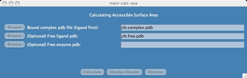
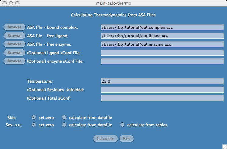
   Because our system type is binding, we enter the bound complex pdb file and optionally enter the free ligand and free enzyme pdb files.

   Note: If the system type was "oligomerization", we enter the bound oligomer pdb and an optional free monomer pdb. For the "unfolding" system type, you enter both the folded and unfolded pdb files.

   • Click the "Calculate" button.

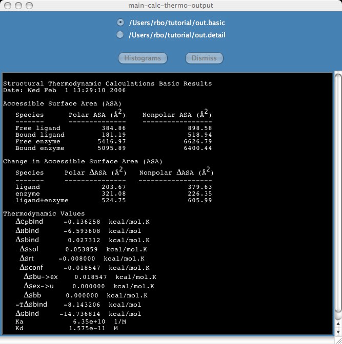
     The program prints a number of messages to the screen telling you what it is doing. The final message should say "Done calculations, no errors".

   • Click the "Display Results" button.

     

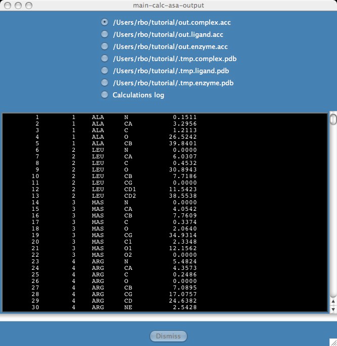
     A results window is displayed which allows you to view the various output files. All accessible surface area output files have the ".acc" file suffix. The log file is important because it indicates all the steps and programs used to derive the ".acc" files and it indicates the nature of any errors. Here are examples of an acc file and a log file. When you are done, click on the "Dismiss" buttons until you arrive back at the first stc window.

4. Click the "Thermodynamics" button.

   

   In this window we make thermodynamics calculations based on accessible surface area files. Note that stc fills in the "ASA file" fields but the user can create or edit his/her own. The other fields are set such that stc calculates sConf in a reasonable way. If you want to change how stc calculates sConf from the default method, see calculating sConf.

5. Click the "Calculate" button.

   

   The program displays a basic output file of various binding constants and other key variables. If you click on the detailed output file you can see thermodynamic output on specific atoms or residues. Here is where you can study the individual atom differences, the classification of polar/nonpolar atoms, a residue by residue summary in the calculation of sconf (including the change in ASA for total polar and non-polar atoms) and the calculation of themodynamic paramaters per residue.

6. Click the "Histograms" button.

   

   Finally, in order to analyze this output more easily, you can click on the "Histograms" button where you can receive graphical displays of the key thermodynamic indicators residue by resiude. Clicking on the radio button automatically draws the requested histogram.

   Notes: Unfortunately I am not able to have the histogram redraw automatically when you resize the window, thus i have a "fit to window" button which does it. I'm sure with a bit of patience, this could be eliminated. Another bug is that the histogram does not know what to do when the residue Ids are not unique. Probably a future version of this software will have options to select the appropriate chain.

7. Click the "Save Postscript".

   Creates a postscript file of the plot. Remember that you have control of the colors, titles, line widths, tics, of your histogram through the stcDefaults file and that you have the ability to re-locate any text via click/drag.

Back to stc home page

This file last updated: