
|
PENCE / CIHR-Group
|

|
Funding for this software has been provided in part by the
Canadian Institutes of Health Research (CIHR Group)
and the
Protein Engineering Networks of
Centres of Excellence (PENCE).
|
|
PENCE / CIHR-Group
|
|
Funding for this software has been provided in part by the
Canadian Institutes of Health Research (CIHR Group)
and the
Protein Engineering Networks of
Centres of Excellence (PENCE).
Purpose: a graphical X-windows program for binding curve studies and NMR spectroscopic analysis.
The power of xcrvfit lies in its convenience to process multiple datasets of various formats, the ability to experiment with fitting parameter scenarios, and the ability to customize the graphics. The program runs quickly and on any platform supporting X-windows. Output from the program includes a graph of the function through the data (saved in postscript format), the rmse of the fit, a measure of the sensitivity of each fitting function parameter, and a table showing how each datapoint fits the function.
The xcrvfit program is a combination of 3 programs previously written in sunview: crvfit, jfit, and t1t2fit.
xcrvfit: a graphical X-windows program for binding curve studies and NMR
spectroscopic analysis, developed by Boyko, R. and Sykes, B.D.  (University of Alberta).
website: http://www.bionmr.ualberta.ca/bds/software/xcrvfit
We are very grateful to the many people who have suggested mathematical equations for use in xcrvfit.
Copyright (C) 1994 - No portion of this program may be incorporated into other programs or sold for profit without express written consent of the authors.
X11 (unix,linux): xcrvfit v3.0.6 (0.50 MB)
If this did not work, it may be because you do not have tcl/tk for your
mac. Install tcl/tk at
http://www.maths.mq.edu.au/~steffen/tcltk/TclTkAqua/
Once you have downloaded the software, you then proceed by
untarring the files if your browser has
not already done so. For example:
If you do not get a graphical window, check with your system administrator
to make sure the program has been installed and is accessible to you.
The default fonts, colors, sizes of the xcrvfit gui are set in the
xcrvfitDefaults file of the current directory.
Click here to see an example.
The program proceeds to read in the data and display the first
data set. If the data is not drawn in the plotting window make
sure you may have data formatting issues.
The program starts by reading the first dataset, but the user
can select another. The user has the choice of changing the offset
for the x data (this is particularly useful for the chemical shift
functions). Finally, the user may want to change how the graph is
displayed in the plotting window by clicking the "Change Graphics"
menu button under options. Here the user can change variables such
as xMax, number of tic marks, titles, colors, etc.
For a more detailed explanation of the functions see
Fitting Functions .
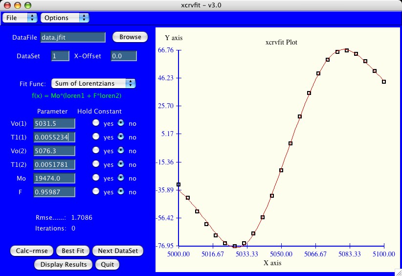
Once the function has been selected, the program displays the
appropriate parameter fields.
A graph of the fitting
function is displayed along with a rmse (root mean square error) value.
If you do not see the fitting function, it could be that your starting
parameters are not very close. Try adjusting the x/y scale to display
a bigger plot (see menubar options/change graphics).
Some functions will converge to the best fit function regardless of
the starting parameters. Others are very sensitive and a close
approximation is required first.
Here you can see how every datapoint corresponds to the fitting
function. Also, you can see how sensitive each fitting parameter
is by looking at the stddev field.
The program then reads in the next dataset. The previous starting
parameters are not erased so that the user may be able to quickly
process several datasets by alternating between "Best Fit" and
"Next Dataset".
kay - In this format the x-values are placed on the first line
and each subsequent line contains an identifier (likely the amino acid
number) and the corresponding y-values.
Any entry preceded with a "#" is treated as a missing value in
the table.
An example of this format is found in the file
data-t2.kay
of the installed lib/examples directory.
jfit - jfit format refers to Varian's vnmr 'fitspec.data' file
format. An example of this format follows below:
Download
Select the version of xcrvfit corresponding to your operating system.
MacOSX (aqua): xcrvfit v3.0.6 (0.30 MB)
Installation
Mac OSX
Your browser will probably already un-tar the download
file. You should be able to double click on the xcrvfit icon for
mac os aqua. Eventually move the xcrvfit icon to /Applications.
X11/unix
	> tar xvf xcrvfit-v3.0.6-build.tar
	> cd xcrvfit-v3.0.6-build
Look at the README file for details on installation. The installation
script is simple, it will ask where you want to install the software.
> ./Install
The README file also explains
how to set your path environment variable to include the location
of the executable. For example, here is what I did on my linux account:
	setenv XCRVFIT_HOME /home/rbo/xcrvfit-v3.0.6
	alias xcrvfit /home/rbo/xcrvfit-v3.0.6/sbin/xcrvfit
Basic Usage of xcrvfit
Input Data Files for xcrvfit
The xcrvfit program can read data files which are in
one of the following formats:
Data which is in the kay, jfit or fp
formats is converted to crvfit
format automatically by the software. Here is a description of
each format type with examples.
crvfit - Each line in the text file contains one point
where the point is specified as either "x f(x)" or "x f(x) x2".
Comments are prefixed by "!".
	! This is a crvfit data file
	!
	! x     f(x)
	!
	1.0    5.1
	2.2    12.0
	3.6    19.3
Multiple datasets can be placed in one file however an ID number
must be found on the line preceding each data set.
An example of this format is found in the file
data-line
of the installed lib/examples directory.
Here is
another example
of where f(x) is dependent on x and x2.
	100  (number of points)
	-20  (start of plot)
	30   (width of plot)
	1.00 (first y-value)
	1.05 (second y-value)
	...
An example of this format is found in the file
data.jfit
of the installed lib/examples directory.
fp - fp format refers to Varian's vnmr 'fp.out' file format.
An example of this format is found in the file
data.fp
of the installed lib/examples directory.
The log file "xcrvfit.log" contains a record of each convergence
achieved through pressing the iterate button. This is particularly
useful for stepping through a number of T2 fits.
Here is an example results file.
Understanding the Output
Data Input.: data.cubic
Num of data: 10

Function...: Cubic Polynomial
Description: Notes: A0*x*x*x + A1*x*x + A2*x + A3
Parameters.: 4

Parameter   Hold Constant          Value         StdDev
A0.......:       no             -0.00506        0.00211
A1.......:       no              1.30573        0.13435
A2.......:       no             -5.14197        2.32052
A3.......:       no              8.09954       10.43368

Stddev.....: 9.5043
Iterations.: 116
Max It.....: 200

Point by Point Analysis
          X[i]           Y[i]         Y-Calc       Residual
       0.00000        2.00000        8.09954        6.09954
       4.30000       13.00000        9.72971       -3.27029
       9.60000       93.00000       74.59546      -18.40454
      14.70000      190.00000      198.59236        8.59236
      18.70000      319.00000      335.45210       16.45210
      23.30000      537.00000      533.14359       -3.85641
      27.50000      750.00000      748.90418       -1.09582
      32.40000     1044.00000     1040.07185       -3.92815
      36.80000     1340.00000     1334.93300       -5.06700
      41.80000     1700.00000     1704.96881        4.96881
Fitting Functions in xcrvfit
Pierre Lavigne has suggested a number of functions in xcrvfit.
These notes are available here.
f(x) = A0*x + A1
f(x) = A0*x^2 + A1*x + A2
f(x) = A0*x^3 + A1*x^2 + A2*x + A3
f(x) = A0 * exp(A1 * x) + A2
f(x) = A0 * (1.0 - A1 * exp(-x / A2))
f(x) = A0 * exp(-x / A1)
f(x) = (A0 * exp(-x / A1)) + (A2 * exp(-x / A3))
f(x) = (A0 * (1 - exp(-x / A1))) + (A2 * (1 - exp(-x / A3)))
	b = 10^((-x)*A3)
	c = 10^((-A0)*A3)
	f(x) = A1 + (b / (b + c)) * (A2 - A1)
f(x) = (A0 * cos(x)^2) - (A1 * cos(x)) + A2
f(x) = (A0 * cos(A1 * x + A2) + A3
f(x) = A0 * cos(2.0*A1) + sin(2.0*A2)
f(x) = A0 + A1 / (1 + exp(-(x - A2) / A3)))
	c = A0 * exp(A1 * A2 * (x - A3));
	d = A0 * A0 * A4 * exp(A1 * A2 * 2.0 * (x - A3));
	f(x) = c + d;
	b = x + 273.15
	c = b *((A4 / A6) + A5 * log(b / A6))
	d = A4 + A5 * (b - A6)
	e = (d - c) / 0.001987
	f = exp((-e) / b)
	g = f / (1 + f)
	f(x) = (1 - g) * (A0 - A1 * x) + g * (A2 - A3 * x)
	b = x + 273.15
	c = b*((A4 / A6) + A5 * log(b/ A6) + 0.001987 * log(A7))
	d = A4 + ( A5 * (b - A6))
 	e = d - c
	f = exp((-e) / (b * 0.001987))
	g = (-f + sqrt((f*f) + 8.0 * A7 * f)) / (4.0 * A7)
	f(x) = (1.0 - g) * (A0 - A1 * x) + g * (A2 - A3 * x)
	b = x + x2 + A1
	f(x) = A0 * (b - sqrt(b*b - 4*x*x2)) / (2.0 * x2)
	b = A3 - 4 * A1
	c = A3 * A3
	d = (c - (4*A1*A3) - (2*x2*A3)) / b
	e = ((x * A3 * (2*x2 - x)) - (c * (x2 + A1 + x))) / b
	f = -(2*d*d*d - 9*d*e + (27 * ((x*x2*c) / b))) / 54.0
	g = (3*e - d*d) / 3.0
	w = f / sqrt(-(g*g*g) / 27.0)
	h = 180.0 / PI * acos(w)
	x3 = (2 * sqrt(-g/3.0) * cos(((h/3.0)+240)*TO_RAD) - (d/3.0))
	f(x) = ((A0*x3) + (A2*x3*(x-x3)/(2*x3+A3))) / x2
	b = 4 * PI * PI
	c = T1(1) / (1 + b*(x-Vo(1))*(x-Vo(1)) * (T1(1)*T1(1))
	d = T1(2) / (1 + b*(x-Vo(2))*(x-Vo(2)) * (T1(2)*T1(2))
	f(x) = Mo * (c + F*d)
	b = (x - a[0]) / a[1];
	lz1 = (1.0 / (2.0 * PI * a[1])) * exp(-0.5 * b * b);
	b = (x - a[2]) / a[3];
	lz2 = (1.0 / (2.0 * PI * a[3])) * exp(-0.5 * b * b);
	f(x) = a[4] * (lz1 + a[5]*lz2);
	b = 4.0 * PI * PI;
	c = 2.0 * PI * a[1] * a[1] * (x-a[0]);
	lz1 = c / (1 + b * (x-a[0])*(x-a[0]) * (a[1]*a[1]));
	c = 2.0 * PI * a[3] * a[3] * (x-a[2]);
	lz2 = c / (1 + b * (x-a[2])*(x-a[2]) * (a[3]*a[3]));
	f(x) = (a[4] * (lz1 - a[5]*lz2));
	set b [expr exp((0.0 - $Parms(4) + $Parms(5) * $x) / $Parms(7))]
	set c [expr abs($b / (3.0 * $Parms(6) * $Parms(6)))]
	set d [expr 0.5 * $c]
	set e [expr sqrt($c * $c * (0.25 + 0.03704 * $c))]
	set g [expr $d + $e]
	set h [expr $d - $e]
	set w [expr pow($g, 0.3333333) - pow(abs($h), 0.3333333)]
	return [expr (1.0 - $w) * ($Parms(0) - $Parms(1) * $x) + $w * ($Parms(2) - $Parms(3) * $x)]
	set b [expr exp((0.0 - $Parms(4) + $Parms(5) * $x) / $Parms(7))]
	set c [expr abs($b / (3.0 * $Parms(6) * $Parms(6)))]
	set d [expr 0.5 * $c]
	set e [expr sqrt($c * $c * (0.25 + 0.03704 * $c))]
	set g [expr $d + $e]
	set h [expr $d - $e]
	set w [expr pow($g, 0.3333333) - pow(abs($h), 0.3333333)]
	set f [expr exp((0.0 - $Parms(0) + $Parms(1) * $x) / $Parms(7))]
	return [expr (1.0 - $w) * $Parms(2) + (1.0 - $f / (1.0 + $f)) * $Parms(3)]
	set c [expr $x * 0.008314]
	set d [expr $x * $x * $Parms(7) + $x * $Parms(0) + $Parms(1)]
	set e [expr $x * $x * $Parms(2) + $x * $Parms(3) + $Parms(4)]
	set f [expr (($Parms(4) - $Parms(1))*($x - $Parms(6))) + ((0.50 *
		($Parms(3) - $Parms(0))) * (( $x * $x ) - ($Parms(6) * $Parms(6)))) +
		((0.3333 * ($Parms(2) - $Parms(8))) * (pow($x,3.0) - pow($Parms(6),3.0)))]
	set s [expr (($Parms(4) - $Parms(1))*(log($x) - log($Parms(6)))) +
		(($Parms(3) - $Parms(0)) * ($x - $Parms(6))) + ((0.50 * ($Parms(2) -
		$Parms(7))) * (($x * $x) - ($Parms(6) * $Parms(6))))]
	set g [expr $f + $Parms(5)]
	set h [expr exp(($b * (($Parms(5) / $Parms(6)) + $s) - $g) / $c)]
	set v [expr $h / (1.0 + $h)]
	set w [expr $v * (1.0 - $v) * ($g * $g / ($c * $x))]
	return [expr $d + $w + ($v * $f)]
	set c [expr $x * 0.008314]
	set d [expr $x * $x * $Parms(8) + $x * $Parms(0) + $Parms(1)]
	set e [expr $x * $x * $Parms(2) + $x * $Parms(3) + $Parms(4)]
	set f [expr (($Parms(4) - $Parms(1))*($x - $Parms(6))) + ((0.50 *
		($Parms(3) - $Parms(0))) * (( $x * $x ) - ($Parms(6) * $Parms(6)))) +
		((0.3333 * ($Parms(2) - $Parms(8))) * (pow($x,3.0) - pow($Parms(6),3.0)))]
	set s [expr (($Parms(4) - $Parms(1))*(log($x) - log($Parms(6)))) +
		(($Parms(3) - $Parms(0)) * ($x - $Parms(6))) + ((0.50 * ($Parms(2) -
		$Parms(8))) * (($x * $x) - ($Parms(6) * $Parms(6))))]
	set g [expr 2.0 * ($f + $Parms(5))]
	set h [expr exp(($x * 2.0 * (($Parms(5) / $Parms(6)) + $s +
		0.008314 * log(1.66 * $Parms(7))) - $g) / $c)]
	set v [expr (( -1.0 * $h + sqrt($h * $h + 8.0 * $Parms(7) * $h)) / (4.0 * $Parms(7)))]
	set w [expr ($v * (1.0 - $v) / (2.0 - $v)) * (2.0 * $g * $g / ($c * $x))]
	return [expr $d + $w + ($v * ($e - $d))]
	set c [expr $x * 0.008314]
	set d [expr $x * $x * $Parms(8) + $x * $Parms(0) + $Parms(1)]
	set e [expr $x * $x * $Parms(2) + $x * $Parms(3) + $Parms(4)]
	set f [expr (($Parms(4) - $Parms(1))*($x - $Parms(6))) + ((0.50 * ($Parms(3) - $Parms(0))) * (( $x * $x ) - ($Parms(6) * $Parms(6)))) + ((0.3333 * ($Parms(2) - $Parms(8))) * (pow($x,3.0) - pow($Parms(6),3.0)))]
	set s [expr (($Parms(4) - $Parms(1))*(log($x) - log($Parms(6)))) + (($Parms(3) - $Parms(0)) * ($x - $Parms(6))) + ((0.50 * ($Parms(2) - $Parms(8))) * (($x * $x) - ($Parms(6) * $Parms(6))))]
	set g [expr $f + $Parms(5)]
	set h [expr exp($x * (($Parms(5) / $Parms(6)) + $s + 0.008314 * log(2.09 * $Parms(7)*$Parms(7)) - $g) / $c)]
	set i [expr sqrt(1.0 + ($h / (20.25 * $Parms(7)*$Parms(7))))]
	set j [expr ($h / (6.0 * $Parms(7)*$Parms(7))) * (1.0 + $i)]
	set k [expr ($h / (6.0 * $Parms(7)*$Parms(7))) * (1.0 - $i)]
	set v [expr pow($j, 0.3333333) + pow($k, 0.3333333)]
	set w [expr ($v * (1.0 - $v) / (3.0 - 2 * $v)) * (3.0 * $g * $g / ($c * $x))]
	return [expr $d + $w + ($v * ($e - $d))]
	set j [expr 8.314 * $Parms(7)]
	set k [expr exp((0.0 - ($Parms(4) + $Parms(5)*$x)) / $j)]
	set m [expr $Parms(2) + $Parms(3) * $x]
	set n [expr ($Parms(0) + $Parms(1) * $x) - $m]
	set p [expr sqrt($k * $k + 8.0 * $Parms(6) * $k)]
	return [expr ($n * ($p - $k)) / (4.0 * $Parms(6)) + $m]
Just take a look at your $HOME/.xcrvfitDefaults file and change it to something better. When you change an item, make sure you don't introduce additional blanks at the end.
Make sure to press return after entering each parameter. If you still don't see a fitting curve then double check the starting parameters, perhaps we are using different units or a different scale for the parameters.
Some functions are very sensitive to the iterative approach. Try holding some of the parameters "constant" before iterating.
Also, some functions require a reasonably close fit to the data before the iterate function can work.
I am willing to look at adding new functions, send me an email.
Crvfit is frequently used in the lab for binding curve studies where some functions are of the form f(x, x2). We have also used crvfit to calculate T1 and T2 relaxation curves and J coupling constants.
When convergence is not easily obtainable (some functions are very sensitive to pertubations), the user can still obtain useful fits by holding parameters constant.
The main disadvantage of crvfit is that it runs on sunview which the lab still supports (but just barely). crvfit was eventually ported to X-windows and is now called xcrvfit.
This file last updated: Questions to: bionmr@biochem.ualberta.ca